2nd LPT Challenge Case 1 Dataset
This page details the test case principle and instructions. Pulished results are presented there.
1. Physical situation
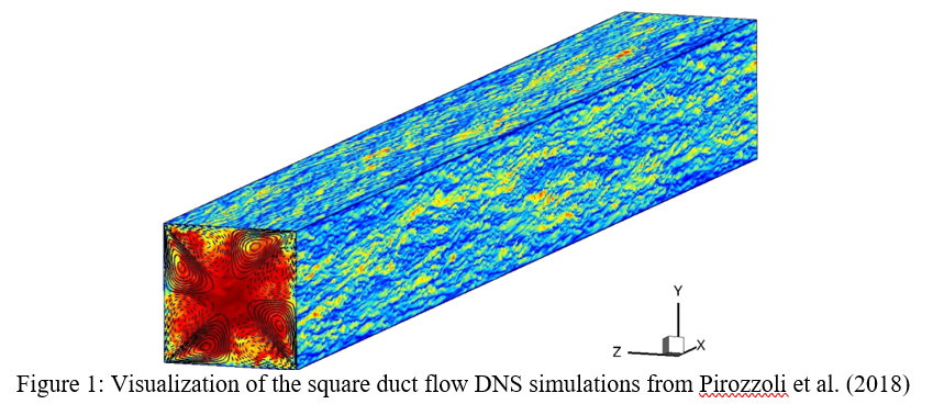
This test case considers the square duct DNS simulations of Pirozzoli et al. (2018), to study a fully developed turbulent flow. The figure below illustrates the simulation results, conducted at a bulk Reynolds number of Reb = 2hub/nu = 40,000 and a friction Reynolds number Retau approximately equal to 1,000, where h denotes the duct half-width, ub is the bulk velocity and nu the fluid’s kinematic viscosity.
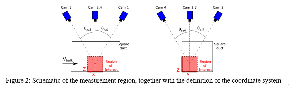
For the challenge, a domain of h x h x h is considered, where x denotes the streamwise direction, and y = 0 and z = 0 are the duct walls. A virtual experiment is conducted in water (rho = 1000 kg/m3, nu = 1 . 10-6 m2/s), with h = 100 mm and ub = 0.2 m/s. The experimental setup is sketched below, including the four-camera arrangement for the LPT challenge. A cloud of virtual particles, hypothesized as fully passive tracers, has been propagated within the DNS simulation.
2. Input data
This test case of the LPT challenge considers four cameras viewing the fully-illuminated measurement region of 100 x 100 x 100 mm. The cameras view the measurement volume mainly from above (z-direction). The cameras (1,024 x ,024 pixels, 10 µm pitch) are located at a height of about z = 1 m with a viewing angle of theta = +/- 30° relative to the z axis. Equipped with f = 105 mm objectives and aiming at the centre of the measurement domain, the full volume is not entirely in view by each camera.
Camera calibration
Camera calibration can be performed by downloading the ASCII file LPT_CASE01_CalibPoints.txt. Each line of this file contains the coordinates of a point in the domain together with its projections on the four cameras:
X Y Z x1 y1 x2 y2 x3 y3 x4 y4
where (X,Y,Z) are the point coordinates in units of mm and (xi,yi) the coordinates of its projection on camera i in units of pixel. Pixel position (0,0) corresponds to the centre of the pixel located at the top left corner of an image.
Cases and images
This test case comprises three different situations, with varying particle displacements in the bulk. The time separation between frames is set to 5.916, 8.283 and 10.649 ms for each case, such that particles at the bulk velocity displace approximately 10, 15 and 20 pixels respectively. For every condition, the seeding density is kept constant at 0.1 ppp. Some typical camera noise is added to the images. A constant particle image size (PSF or OTF) is used. A sequence of 100 frames (starting at frame 0) is provided for each situation, and the images are stored in 16-bit tiff compressed format.
The images are named in the following format:
LPT_CASE01_TR_dtT_IBBBB_C.tif, with:
T: dt value (1, 2 or 3), corresponding to the approximate bulk displacement of 10, 15 and 20 px respectively
BBBB: snapshot number, starting from 0000
C: camera number, from 0 to 3
3. Requested output and formatting rules for upload
3.1. Mandatory cases
Results for all values of parameter dt should be provided. Each file should contain information about the flow field for time step 49 (from the sequence starting at 0).
3.2. Preparing your upload
Please replicate the contents of the sample archive myAlgo_LPT_CASE01.zip:
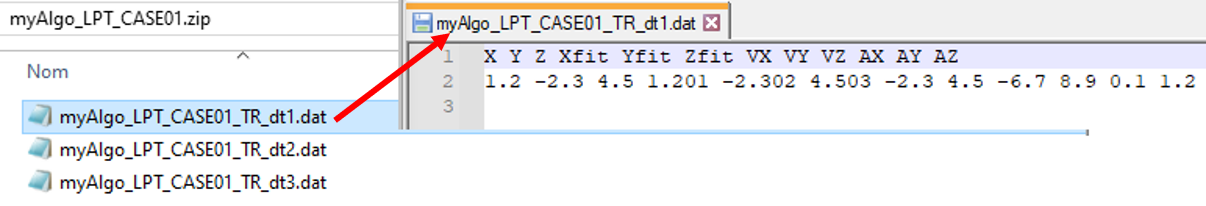
- Results for each time separation should be stored in an ASCII file with first line equal to X Y Z Xfit Yfit Zfit VX VY VZ AX AY AZ followed by one line for each particle track with raw position X, Y, Z in mm, fitted position (i.e. associated to the estimation of velocity and acceleration) Xfit, Yfit, Zfit in mm, the velocity VX, VY, VZ in m/s, and the acceleration AX, AY, AZ in m/s2, all calculated at time step 49 (independently of the time separation). There is no specific convention about number formatting.
- File naming convention (as above): myAlgo_LPT_CASE01_TR_ppp_0_AAA.dat, with AAA the fractional value of seeding density in ppp and "myAlgo" a string that can be chosen freely, but without any space in it.
- Once your files are ready, as in the example above, please zip them directly into a single archive. Please make sure that you do not zip a folder containing the results, as this will result in the submission being rejected.
3.3. Upload form
Once your zip archive is ready, clicking on "Submit TP results" or on "Submit TR results" will open a form allowing you to upload a file containing your results.
The upload form should also be filled with the following information, which is used for result presentation only if you choose to publish your result based on the evaluation sent by email:
- List of authors (default: submitter name)
- Authors' institution(s) (default: submitter institution)
- Optional: departement / team (default: submitter's departement / team)
- Algorithm's short name or acronym
- Algorithm's full name
- Optional: URL address of the publication on your algorithm, or of a webpage describing it
For these fields, note that rules apply, in terms of maximum length and/or authorized characters. These are displayed on the form in the explanatory text of each field. In particular, commas are not allowed in any of the above fields.
Contact in case of any questions: Andrea Sciacchitano, TU Delft: a.sciacchitano@tudelft.nl
References
Pirozzoli, S., Modesti, D., Orlandi, P., & Grasso, F. (2018). Turbulence and secondary motions in square duct flow. Journal of Fluid Mechanics, 840, 631–655. doi:10.1017/jfm.2018.66