2nd DA Challenge Case 1 Datasets | ONERA flow reconstruction benchmarks

2^nd DA Challenge Case 1 Datasets

This page details the test case principle and instructions. To see published results, see the corresponding pages for two-pulse, four-pulse and time-resolved cases.

1. Physical situation

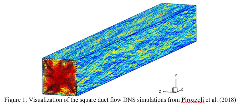
This test case considers the square duct DNS simulations of Pirozzoli et al. (2018), to study a fully developed turbulent flow. The figure below illustrates the simulation results, conducted at a bulk Reynolds number of Re_b = 2hu_b/nu = 40,000 and a friction Reynolds number Re_tau approximately equal to 1,000, where h denotes the duct half-width, u_b is the bulk velocity and nu the fluid’s kinematic viscosity.

For the challenge, a domain of h x h x h is considered, where x denotes the streamwise direction, and y = 0 and z = 0 are the duct walls. A virtual experiment is conducted in water (rho = 1000 kg/m³, nu = 1 . 10^-6 m²/s), with h = 100 mm and u_b = 0.2 m/s. The experimental setup is sketched below, including the four-camera arrangement for the LPT challenge. A cloud of virtual particles, hypothesized as fully passive tracers, has been propagated within the DNS simulation.

2. Input data

This test case of the DA challenge consists of the reconstruction of the velocity and pressure fields from scattered positions of particles. Simulated results from time-resolved (TR) acquisitions, four-pulse (FP) recordings and two-pulse (TP) recordings are considered. For each, seeding density is varied over 0.001 ppp, 0.01 ppp, 0.05 ppp and 0.2 ppp.

The particles’ positions in 3D space and the particles’ IDs are given in ASCII files. The first three columns of the data files correspond to the instantaneous X, Y, Z particle coordinates respectively (given in mm). The particles within the same track are identified with the particles/track ID (4^th column). The data files have a header composed by three lines:

Title = Snapshot #
Variables = X Y Z PartID
Zone I= , F=POINT

The parameter I indicates the number of particles present in Snapshot #n.

2.1. TR cases

A sequence of 50 consecutive frames (starting at 0) is provided for each seeding density case. The time separation between snapshots is 5.916 ms. The file naming follows the convention:

DA_CASE01_TR_ppp_0_AAA_PartFile_BBBB.dat

where AAA is the fractional value of the seeding density in ppp (e.g. 010 for 0.01 ppp images), and BBBB is the snapshot number (from 0000 to 0049).

2.2. FP cases

The particles belonging to each of the four pulses of the sequence are provided for every seeding density case. The timing template of the four-pulse acquisition is 2-1-2, with the unitary separation of 5.916 ms. This means that the time separation between the first and second pulse is 11.832 ms, the separation between the second and third pulses is 5.916 ms, and finally between the third and fourth pulses is again 11.832 ms. The file naming follows the convention:

DA_CASE01_FP_ppp_0_AAA_PartFile_BBBB.dat

where AAA is the fractional value of the seeding density in ppp (e.g. 001 for 0.001 ppp images), and BBBB is the pulse number (from 0000 to 0003).

2.3. TP cases

The particles belonging to each of the two pulses of the sequence are provided for every seeding density case. The time separation between pulses is 5.916 ms. The file naming follows the convention:

DA_CASE01_TP_ppp_0_AAA_PartFile_BBBB.dat

where AAA is the fractional value of the seeding density in ppp (e.g. 200 for 0.2 ppp images), and BBBB is the pulse number (from 0000 to 0001).

3. Requested output and formatting rules

3.1. Requested data and file formatting

The results need to be prescribed on a Cartesian grid with constant spacing of 1 mm in each direction. The following ranges are requested:

X: 101 grid points, from x = 0 to x = 100 mm
Y: 100 grid points, from y = 0.1 to y = 99.1 mm
Z: 100 grid points, from
z = 0.1 to z = 99.1 mm

corresponding to a total number of 1,010,000 grid points.

The output variables required on this grid are the following (total of 13 variables):

Velocity components: VX, VY, VZ in m/s
Velocity gradient components: dVXdX, dVXdY, dVXdZ, dVYdX, dVYdY, dVYdZ, dVZdX, dVZdY, dVZdZ in 1/s
Static pressure: p in Pa

where the pressure variable refers to the relative pressure with respect to the point (X,Y,Z) = (0,0.1,0.1) mm.

In order to ease file transfer, output files are requested in HDF5 format. In order to avoid confusion, the space coordinates are expected to vary in the order: X, Y and then Z, i.e. X corresponding to the innermost loop and Z to the outermost loop.

Sample scripts generating such .h5 files with the expected format are available for download in Matlab and Python. Note that they in fact correspond to the case of the First DA challenge held in 2020, so they should be adapted e.g. in terms of number of mesh points.

3.1.1. TR cases

The flow field at timestep 24 (from the sequence starting at 0) needs to be supplied for each seeding density situation. Providing the output also at timestep 2 is optional. The file name has to follow:

ZZZZ_DA_CASE01_TR_ppp_0_AAA_PartFile_BBBB.h5

where XXXXX corresponds to the acronym / short name of your algorithm (3 characters minimum, no space, only [A-Z0-9a-z]_-@ chars) as indicated in the corresponding field of the upload form (i.e. both should match, including for upper and lower case letters), AAA is the fractional value of the seeding density in ppp (e.g. 001 for 0.001 ppp images) and BBBB is the snapshot number (e.g. 0002 or 0024). ZZZZ is a free string to identify your result (free number of characters), but should contain no space.

3.1.2. FP cases

The flow field at the time in the middle of the second and third pulses (centre of the sequence) needs to be supplied for each seeding density situation. The file name has to follow:

ZZZZ_DA_CASE01_FP_ppp_0_AAA.h5

ZZZZ is a free string to identify your result (free number of characters), but should contain no space.

3.1.3. TP cases

The flow field at the time in the middle of the two pulses needs to be supplied for each seeding density situation. The file name has to follow:

ZZZZ_DA_CASE01_TP_ppp_0_AAA.h5

where XXXXX corresponds to the acronym / short name of your algorithm (3 characters minimum, no space, only [A-Z0-9a-z]_-@ chars) as indicated in the corresponding field of the upload form (i.e. both should match, including for upper and lower case letters), AAA is the fractional value of the seeding density in ppp (e.g. 001 for 0.001 ppp images). ZZZZ is a free string to identify your result (free number of characters), but should contain no space.

3.2. Preparing your upload

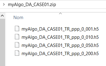
Once your .h5 files are produced, please make sure that you zip them directly (do not zip a folder containing them, as this will result in the submission being rejected) into a single archive, as in the example of myAlgo_DA_CASE01.zip below:

3.3. Upload form

Once your zip archive is ready, clicking on "Submit TP results", "Submit FP results" or on "Submit TR results" will open a form allowing you to upload a file containing your results.

The upload form should also be filled with the following information, which is used for result presentation only if you choose to publish your result based on the evaluation sent by email:

List of authors (default: submitter name)
Authors' institution(s) (default: submitter institution)
Optional: departement / team (default: submitter's departement / team)
Algorithm's short name or acronym
Algorithm's full name
Optional: URL address of the publication on your algorithm, or of a webpage describing it

For these fields, note that rules apply, in terms of maximum length and/or authorized characters. These are displayed on the form in the explanatory text of each field. In particular, commas are not allowed in any of the above fields.

Contact in case of any questions: Adrian Grille Guerra and Andrea Sciacchitano, TU Delft: A.GrilleGuerra@tudelft.nl, a.sciacchitano@tudelft.nl

References

Pirozzoli, S., Modesti, D., Orlandi, P., & Grasso, F. (2018). Turbulence and secondary motions in square duct flow. Journal of Fluid Mechanics, 840, 631–655. doi:10.1017/jfm.2018.66