2nd LPT Challenge Case 3 Datasets
This page details the test case principle and instructions. To see published results, see the corresponding pages for two-pulse and time-resolved cases.
1. Physical situation and input data
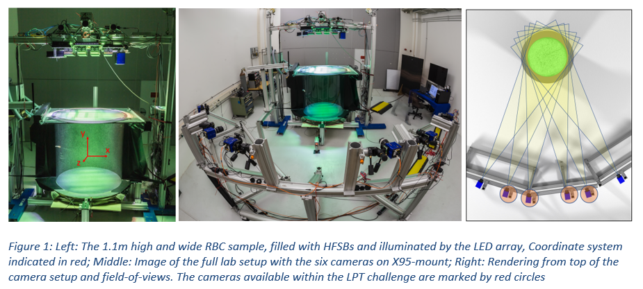
The experimental dataset comprises images of Helium-filled soap bubbles within a Rayleigh-Bénard convection cell, captured by four (out of six) 5.5 MegaPixel SCMOS cameras (Bosbach et al. 2021, Godbersen et al. 2021, Weiss et al. 2024). The experiment was conducted at DLR Göttingen and consisted of an electrically heated aluminum plate and a water-perfused cooling plate, which allows for illumination from the top using an assortment of LED arrays (see Fig. 1). A total of six PCO edge 5.5 SCMOS cameras (2560 × 2160 pixels with a 6.5 µm pitch and an average magnification of 1.8942 px/mm) was installed and equipped with Zeiss Distagon 35 mm lenses. They were installed at the height of the upper cooling plate and slightly tilted downwards to view the full cell. Despite the strong reflection on the black bottom plate, bubbles are still visible in this region. The flow was recorded at a repetition rate of 30 Hz for over 30 minutes. The images captured by all six cameras over 54528 time-steps were used to reconstruct Lagrangian Particle Tracks using the DLR Shake-The-Box implementation; these results will serve as a Ground Truth for the evaluation of the LPT challenge results. For the challenge data, the four inner cameras of the in-line camera setup are selected (marked in red in Fig. 1, right), all viewing the entire volume within the cell. The omission of the two outer cameras severely aggravates the reconstruction problem, allowing the six-camera solution to be regarded as a Ground Truth.
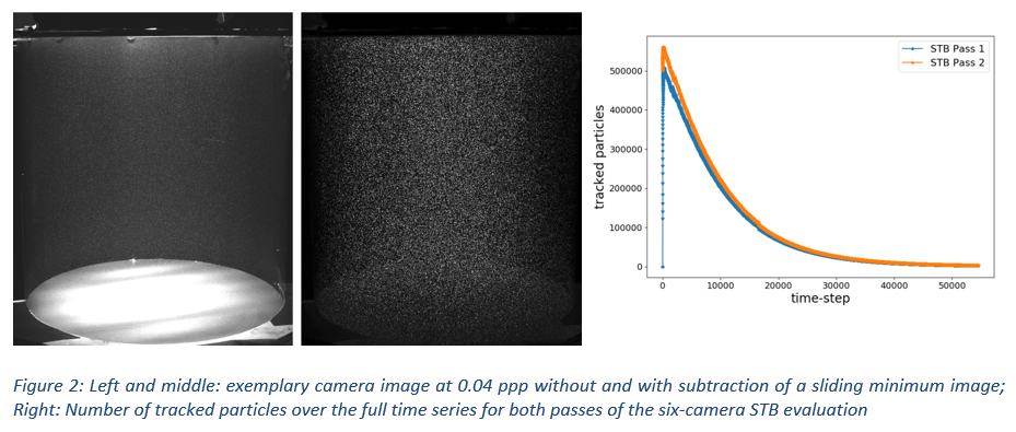
The use of Helium-filled soap bubbles with limited lifetime leads to an ever-diminishing particle density over the measurement. This allows to extract short time-series of images at arbitrary particle image density. At the beginning, the six-camera evaluation is able to track around 550,000 bubbles, corresponding to over 0.13 ppp at an assumed active image area of around 4Mpix; at the end of the time-series 2385 tracked bubbles remain (see Fig. 2 right). Please note that the visible particle image density varies greatly over the image due to the circular shape of the sample, therefore the given ppp-values represent averages over the active image.
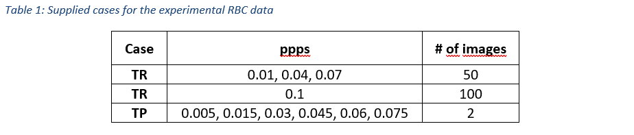
For the reconstructions with only four cameras we supply time-series of 50 images at 0.01, 0.04 and 0.07 ppp and 100 images at 0.1 ppp. Two-pulse-cases are available at 0.005, 0.015, 0.045, 0.06 and 0.075 ppp (see Table 1). The disjoint values for TR and TP are chosen to avoid an overlap of flow situations and images between the two modes. For each case, a sliding minimum image is provided for image preprocessing, created by taking for each pixel the minimum over +/- 10 images of the first image (see Fig. 2).
For calibration, two options are available – either a total of around 75.000 random points within a slightly enlarged reconstruction volume (‘LPT_CASE03_CalibPoints.txt’) or a version with around 14.000 points on several x-y-planes at different z-depths (‘LPT_CASE03_CalibPoints_on_grid.txt’). The point correspondences were created using the fully calibrated two-plane camera model (initial plate calibration, volume self-calibration and finally a B-spline based 2D correction field which accounts for the curvature of the plexiglass) that was used within the six-camera STB evaluation. Participants can either just use these points to calibrate their camera models or additionally perform a Volume-Self-Calibration using the supplied time-series.
The coordinate system is approximately centered in the sample, with X, Y and Z within (-550 to +550, -610 to 500, -550 to +550,) mm. The dynamic range of the velocity is rather high, with low particle shifts in some regions, while the highest velocities can reach around 0.35 m/s, corresponding to a particle shift of around 20 pixels (these values have not been checked for all data points, so they should not be used as absolute limits).
2. Requested output and formatting rules for upload
Participants can choose whether they want to process the TR or the TP data, or both.
2.1. TP case
2.1.1. Mandatory cases
Results have to be submitted at least up to ppp = 0.045. Processing the higher seeded cases is of course encouraged; in that case, all seeding density should be provided up to the highest chosen one.
2.1.2. Preparing your upload
Please replicate the contents of the sample archive myAlgo_LPT_CASE03_TP.zip:
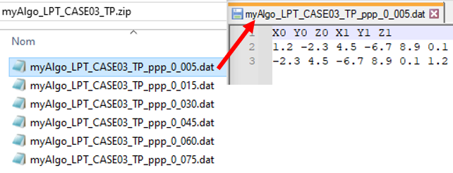
- Results for each seeding density should be stored in an ASCII file with first line equal to X0 Y0 Z0 X1 Y1 Z1 followed by one line for each particle with the two measured particle positions X0, Y0, Z0 and X1, Y1, Z1 in mm for time steps t0 and t1. There is no specific convention about number formatting.
- File naming convention (as above): myAlgo_LPT_CASE03_TP_ppp_0_AAA.dat, with AAA the fractional value of seeding density in ppp and "myAlgo" a string that can be chosen freely, but without any space in it.
- Once your files are ready, as in the example above, please zip them directly into a single archive. Please make sure that you do not zip a folder containing the results, as this will result in the submission being rejected.
2.2. TR case
2.2.1. Mandatory cases
Results have to be submitted at least up to ppp = 0.07. Processing the higher seeded cases is of course encouraged; in that case, all seeding density should be provided up to the highest chosen one.
Important: the requested snapshot number depends on the seeding density value: time step 25 (images ‘_I0024’) shoud be provided for ppp ≤ 0.07, while time step 50 (images ‘_I0049’) is expected for ppp = 0.1.
2.2.2. Preparing your upload
Please replicate the contents of the sample archive myAlgo_LPT_CASE03_TR.zip:
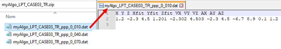
- Results for each seeding density should be stored in an ASCII file with first line equal to X Y Z Xfit Yfit Zfit VX VY VZ AX AY AZ followed by one line for each particle track with raw position X, Y, Z in mm, fitted position (i.e. associated to the estimation of velocity and acceleration) Xfit, Yfit, Zfit in mm, the velocity VX, VY, VZ in m/s, and the acceleration AX, AY, AZ in m/s2, all calculated at time step 40 or 90 depending on the seeding density of the case. There is no specific convention about number formatting.
- File naming convention (as above): myAlgo_LPT_CASE03_TR_ppp_0_AAA.dat, with AAA the fractional value of seeding density in ppp and "myAlgo" a string that can be chosen freely, but without any space in it.
- Once your files are ready, as in the example above, please zip them directly into a single archive. Please make sure that you do not zip a folder containing the results, as this will result in the submission being rejected.
2.3. Upload form
Once your zip archive is ready, clicking on "Submit TP results" or on "Submit TR results" will open a form allowing you to upload a file containing your results.
The upload form should also be filled with the following information, which is used for result presentation only if you choose to publish your result based on the evaluation sent by email:
- List of authors (default: submitter name)
- Authors' institution(s) (default: submitter institution)
- Optional: departement / team (default: submitter's departement / team)
- Algorithm's short name or acronym
- Algorithm's full name
- Optional: URL address of the publication on your algorithm, or of a webpage describing it
For these fields, note that rules apply, in terms of maximum length and/or authorized characters. These are displayed on the form in the explanatory text of each field. In particular, commas are not allowed in any of the above fields.
Contact in case of any questions: Daniel Schanz, DLR: daniel.schanz@dlr.de
Literature
Bosbach J, Schanz D, Godbersen P, Schröder A (2021) Spatially and temporally resolved measurements of turbulent Rayleigh-Bénard convection by Lagrangian particle tracking of long-lived helium-filled soap bubbles, 14th International Symposium on Particle Image Velocimetry
Godbersen P, Bosbach J, Schanz D, Schröder A (2021). Beauty of turbulent convection: a particle tracking endeavor. Physical Review Fluids, 6(11), 110509.
Weiss, S., Schanz, D., Erdogdu, A. O., Schröder, A., & Bosbach, J. (2024). On Lagrangian properties of turbulent Rayleigh–Bénard convection. Journal of Fluid Mechanics, 999, A90.