First DA Challenge datasets
The present page describes the input data as well as rules for submitting results (with corresponding download/upload links in the left panel). For more information about the physical situation, see the First Challenge description page.
Published results can be found on this page.
1. Domain of interest and setup
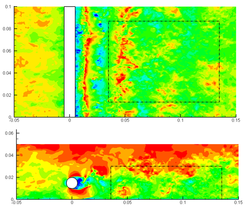
The DA challenge consists of the reconstruction of the velocity fields from scattered positions of particles. The flow test case is the same as for the LPT challenge: the wake of a cylinder embedded in a turbulent boundary layer (free-stream velocity of around 0.7 m/s, momentum thickness Reynolds number Retheta of around 4,500). The dataset comprises particle positions for three cases with different particles concentrations. The positions of the particles are given in the three-dimensional space for a sequence of 50 evenly spaced time instants. The flow domain and the origin of the system of axes for the DA challenge defined as follows (see also figures below):
- Origin of the frame of reference: middle of the volume in X and Y, and located at the plate wall in Z. The origin is 85 mm downstream of the centre of the cylinder.
- Streamwise direction X: between -50 mm and +50 mm (from 35 mm to 135 mm downstream of the centre of the cylinder)
- Wall normal direction Z: between 0 mm (wall location) and 30 mm
Further physical data relevant for the flow situation are: fluid density rho = 998.2 kg/m3 and kinematic viscosity nu = 9.991 10-7m2/s.
2. Input data
The particles’ positions in 3D space and the particles ID are provided to the participants. The first three columns of the data file correspond to the instantaneous X, Y and Z particle coordinates, respectively (given in mm). The particles within the same track are identified with the particles/track ID (4th column). The data file has a header composed by three lines:
1. Title = Snapshot #
2. Variables = “X” “Y” “Z” “PartID”
3. Zone I= , F=POINT
The time separation between successive snapshots (i.e. between Snapshot #n+1 and Snapshot #n) is of 600 ms. The parameter I indicates the number of particles present in Snapshot #n.
Participants are asked to determine all required information for their DA algorithm (e.g. particles velocities and material accelerations) from the provided particle positions.
Each file name is built on model
DA_ppp_0_AAA_PartFile_BBBB.dat
where AAA is the fractional value of the seeding density in ppp (e.g. 025 for the 0.025 ppp case), and BBBB is the snapshot number, with leading zeros. This seeding density corresponds to that of images that would have been obtained from the setup of the 1st LPT challenge.
3. Requested cases and formatting rules for upload
3.1. Mandatory cases
All seeding density cases should be processed and uploaded. For each, the flow field for time step 25 (corresponding to file DA_ppp_0_AAA_PartFile_0025.dat) needs to be supplied.
3.2. Preparing your upload
Please follow the example of fictitious archive "myAlgo_DA.zip" displayed below:
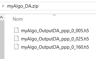
- Results for each seeding density should be stored in an HDF5 file (.h5 extension)
- File naming convention (as above): myAlgo_OutputDA_ppp_0_AAA.h5, with AAA the fractional value of seeding density in ppp and "myAlgo" a string that can be chosen freely, but without any space in it.
- Once your files are ready, as in the example above, please zip them directly into a single archive. Please make sure that you do not zip a folder containing the results, as this will result in the submission being rejected.
Each .h5 file should contain results on the following Cartesian grid, with 0.4 mm spacing in each direction (2,403,576 points total):
- X: 251 points, over interval [-50,50] mm
- Y: 126 points, over interval [-25,25] mm
- Z: 76 points, over interval [0.01,30.01] mm. Location of the first point relative to the wall has been chosen so as to roughly coincide with the first mesh cell of the LES used for the case
This mesh is imposed in order to facilitate the analysis of the results. However, participants are of course encouraged to use the computational mesh for DA that they think most adapted, and then to perform an interpolation on the output mesh.
Variables to be stored in each .h5 files are the following (total 13 variable at each 3D mesh point):
- Velocity components: VX, VY, VZ (in m/s)
- Velocity gradient components: dVXdX, dVXdY, dVXdZ, dVYdX, dVYdY, dVYdZ, dVZdX, dVZdY, dVZdZ (in 1/s)
- Pressure: p (in Pa)
where the pressure variable refers to the relative pressure with respect to point (X,Y,Z) = (0,0.2,0.01), i.e. the value at each mesh point is the local pressure to which the pressure at (X,Y,Z) = (0,0.2,0.01) has been subtracted.
The space coordinates are expected to vary in the order: X, Y and then Z, i.e. X corresponding to the innermost loop and Z to the outermost loop.
Sample scripts generating such .h5 files with the expected format are available for download in Matlab and Python.
3.3. Upload form
Once your zip archive is ready, clicking on "Submit TP results" or on "Submit TR results" will open a form allowing you to upload a file containing your results.
The upload form should also be filled with the following information, which is used for result presentation only if you choose to publish your result based on the evaluation sent by email:
- List of authors (default: submitter name)
- Authors' institution(s) (default: submitter institution)
- Optional: departement / team (default: submitter's departement / team)
- Algorithm's short name or acronym
- Algorithm's full name
- Optional: URL address of the publication on your algorithm, or of a webpage describing it
For these fields, note that rules apply, in terms of maximum length and/or authorized characters. These are displayed on the form in the explanatory text of each field. In particular, commas are not allowed in any of the above fields.
Contact in case of questions: Benjamin Leclaire, ONERA: benjamin.leclaire@onera.fr